【推理引擎】ONNX模型解析

定义模型结构

首先使用 PyTorch 定义一个简单的网络模型：

class ConvBnReluBlock(nn.Module):    def __init__(self) -> None:        super().__init__()        self.conv1 = nn.Conv2d(3, 64, 3)        self.bn1 = nn.BatchNorm2d(64)        self.maxpool1 = nn.MaxPool2d(3, 1)        self.conv2 = nn.Conv2d(64, 32, 3)        self.bn2 = nn.BatchNorm2d(32)            self.relu = nn.ReLU()    def forward(self, x):        out = self.conv1(x)        out = self.bn1(out)        out = self.relu(out)        out = self.maxpool1(out)                out = self.conv2(out)        out = self.bn2(out)        out = self.relu(out)                return out

在导出模型之前，需要提前定义一些变量：

model = ConvBnReluBlock()     # 定义模型对象x = torch.randn(2, 3, 255, 255)      # 定义输入张量

然后使用 PyTorch 官方 API（torch.onnx.export）导出 ONNX 格式的模型：

# way1:torch.onnx.export(model, (x), "conv_bn_relu_evalmode.onnx", input_names=["input"], output_names=['output'])# way2:import torch._C as _CTrainingMode = _C._onnx.TrainingModetorch.onnx.export(model, (x), "conv_bn_relu_trainmode.onnx", input_names=["input"], output_names=['output'],                opset_version=12,                    # 默认版本为9,但是如果低于12，将不能正确导出 Dropout 和 BatchNorm 节点                training=TrainingMode.TRAINING,      # 默认模式为 TrainingMode.EVAL                do_constant_folding=False)           # 常量折叠，默认为True，但是如果使用TrainingMode.TRAINING模式，则需要将其关闭# way3torch.onnx.export(model,                (x),                "conv_bn_relu_dynamic.onnx",                input_names=['input'],                output_names=['output'],                dynamic_axes={'input': {0: 'batch_size', 2: 'input_width', 3: 'input_height'},                            'output': {0: 'batch_size', 2: 'output_width', 3: 'output_height'}})

可以看到，这里主要以三种方式导出模型，下面分别介绍区别：

• way1：如果模型中存在 BatchNorm 或者 Dropout，我们在导出模型前会首先将其设置成 eval 模式，但是这里我们即使忘记设置也无所谓，因为在导出模型时会自动设置（export函数中training参数的默认值为TrainingMode.EVAL）。
• way2：如果我们想导出完整的模型结构，包括 BatchNorm 和 Dropout，则应该将 training 属性设置为 train 模式。
• way3：如果想要导出动态输入的模型结构，则需要设置 dynamic_axes 属性，比如这里我们将第一、三和四维设置成动态结构，那么我们就可以输入任何Batch大小、任何长宽尺度的RGB图像。

下图分别将这三种导出方式的模型结构使用 Netron 可视化：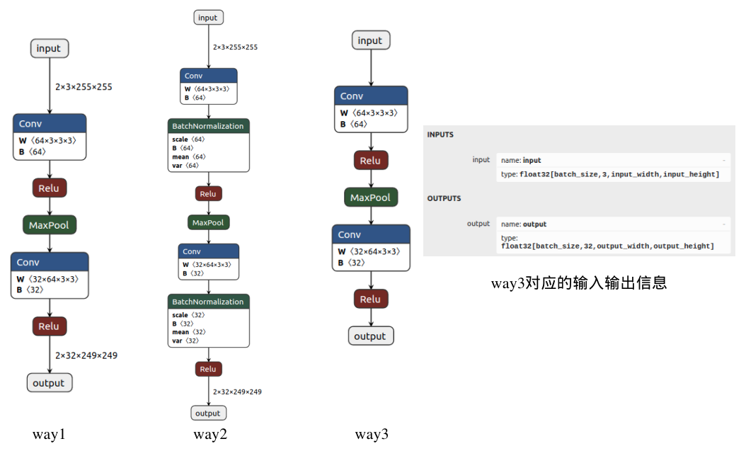

分析模型结构

这里参考了BBuf大佬的讲解：【传送门：https://zhuanlan.zhihu.com/p/346511883】
接下来主要针对 way1 方式导出的ONNX模型进行深入分析。

ONNX格式定义：https://github.com/onnx/onnx/blob/master/onnx/onnx.proto
在这个文件中，定义了多个核心对象：ModelProto、GraphProto、NodeProto、ValueInfoProto、TensorProto 和 AttributeProto。

在加载ONNX模型之后，就获得了一个ModelProto，其中包含一些

• 版本信息(本例中：ir_version = 7)
• 生成者信息：producer_name: pytorch，producer_version: 1.10，这两个属性主要用来说明由哪些框架哪个版本导出的onnx
• 核心组件：GraphProto

在 GraphProto 中，有如下几个属性需要注意：

• name：本例中：name = 'torch-jit-export'
• input 数组：

  [name: "input"type {  tensor_type {    elem_type: 1    shape {      dim {        dim_value: 2      }      dim {        dim_value: 3      }      dim {        dim_value: 255      }      dim {        dim_value: 255      }    }  }}]

• output 数组：

  [name: "output"type {  tensor_type {    elem_type: 1    shape {      dim {        dim_value: 2      }      dim {        dim_value: 32      }      dim {        dim_value: 249      }      dim {        dim_value: 249      }    }  }}]

• node 数组，该数组中包含了模型中所有的计算节点（本例中："Conv_0"、"Relu_1"、"MaxPool_2"、"Conv_3"、"Relu_4"），以及各个节点的属性，：

   [input: "input"input: "23"input: "24"output: "22"name: "Conv_0"op_type: "Conv"attribute {  name: "dilations"  ints: 1  ints: 1  type: INTS}attribute {  name: "group"  i: 1  type: INT}attribute {  name: "kernel_shape"  ints: 3  ints: 3  type: INTS}attribute {  name: "pads"  ints: 0  ints: 0  ints: 0  ints: 0  type: INTS}attribute {  name: "strides"  ints: 1  ints: 1  type: INTS}, input: "22"output: "17"name: "Relu_1"op_type: "Relu", input: "17"output: "18"name: "MaxPool_2"op_type: "MaxPool"attribute {  name: "kernel_shape"  ints: 3  ints: 3  type: INTS}attribute {  name: "pads"  ints: 0  ints: 0  ints: 0  ints: 0  type: INTS}attribute {  name: "strides"  ints: 1  ints: 1  type: INTS}, input: "18"input: "26"input: "27"output: "25"name: "Conv_3"op_type: "Conv"attribute {  name: "dilations"  ints: 1  ints: 1  type: INTS}attribute {  name: "group"  i: 1  type: INT}attribute {  name: "kernel_shape"  ints: 3  ints: 3  type: INTS}attribute {  name: "pads"  ints: 0  ints: 0  ints: 0  ints: 0  type: INTS}attribute {  name: "strides"  ints: 1  ints: 1  type: INTS}, input: "25"output: "output"name: "Relu_4"op_type: "Relu"]

  通过以上 node 的输入输出信息，可提取出节点之间的拓扑关系，构建出一个完整的神经网络。
• initializer 数组：存放模型的权重参数。

  [dims: 64dims: 3dims: 3dims: 3data_type: 1name: "23"raw_data: "\220\251\001>\232\326&>\253\227\372 ... 省略一眼望不到头的内容 ... "dims: 64data_type: 1name: "24"raw_data: "Rt\347\275\005\203\0 ..."dims: 32dims: 64dims: 3dims: 3data_type: 1name: "26"raw_data: "9\022\273;+^\004\2 ..."...

至此，我们已经分析完 GraphProto 的内容，下面根据图中的一个节点可视化说明以上内容：

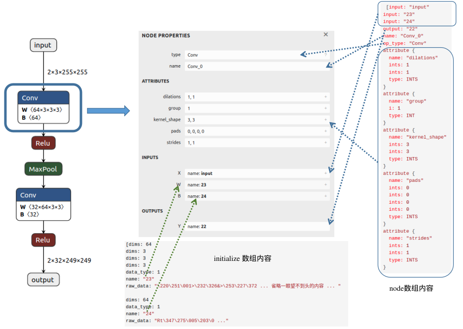
从图中可以发现，Conv 节点的输入包含三个部分：输入的图像（input）、权重（这里以数字23代表该节点权重W的名字）以及偏置（这里以数字24表示该节点偏置B的名字）；输出内容的名字为22；属性信息包括dilations、group、kernel_shape、pads和strides，不同节点会具有不同的属性信息。在initializer数组中，我们可以找到该Conv节点权重（name:23）对应的值(raw_data)，并且可以清楚地看到维度信息（64X3X3X3）。