chapter3——逻辑回归手动+sklean版本

1 导入numpy包

import numpy as np

2 sigmoid函数

def sigmoid(x):    return 1/(1+np.exp(-x))demox = np.array([1,2,3])print(sigmoid(demox))#报错#demox = [1,2,3]# print(sigmoid(demox))

结果：

[0.73105858 0.88079708 0.95257413]

3 定义逻辑回归模型主体

### 定义逻辑回归模型主体def logistic(x, y, w, b):    # 训练样本量    num_train = x.shape[0]    # 逻辑回归模型输出    y_hat = sigmoid(np.dot(x,w)+b)    # 交叉熵损失    cost = -1/(num_train)*(np.sum(y*np.log(y_hat)+(1-y)*np.log(1-y_hat)))     # 权值梯度    dW = np.dot(x.T,(y_hat-y))/num_train     # 偏置梯度    db = np.sum(y_hat- y)/num_train    # 压缩损失数组维度    cost = np.squeeze(cost)    return y_hat, cost, dW, db

4 初始化函数

def init_parm(dims):    w = np.zeros((dims,1))    b = 0    return w ,b 

5 定义逻辑回归模型训练过程

### 定义逻辑回归模型训练过程def logistic_train(X, y, learning_rate, epochs):    # 初始化模型参数    W, b = init_parm(X.shape[1])      cost_list = []      for i in range(epochs):        # 计算当前次的模型计算结果、损失和参数梯度        a, cost, dW, db = logistic(X, y, W, b)            # 参数更新        W = W -learning_rate * dW        b = b -learning_rate * db                if i % 100 == 0:            cost_list.append(cost)           if i % 100 == 0:            print('epoch %d cost %f' % (i, cost))     params = {                    'W': W,                    'b': b    }            grads = {                    'dW': dW,                    'db': db    }     return cost_list, params, grads

6 定义预测函数

def predict(X,params):    y_pred = sigmoid(np.dot(X,params['W'])+params['b'])    y_preds = [1 if y_pred[i]>0.5 else 0 for i in range(len(y_pred))]     return y_preds

7 生成数据

# 导入matplotlib绘图库import matplotlib.pyplot as plt# 导入生成分类数据函数from sklearn.datasets import make_classification# 生成100*2的模拟二分类数据集x ,label  = make_classification(    n_samples=100,# 样本个数    n_classes=2,# 样本类别    n_features=2,#特征个数    n_redundant=0,#冗余特征个数（有效特征的随机组合）    n_informative=2,#有效特征，有价值特征    n_repeated=0, # 重复特征个数（有效特征和冗余特征的随机组合）    n_clusters_per_class=2 ,# 簇的个数    random_state=1,)print("x.shape =",x.shape)print("label.shape = ",label.shape)print("np.unique(label) =",np.unique(label))print(set(label))# 设置随机数种子rng = np.random.RandomState(2)# 对生成的特征数据添加一组均匀分布噪声https://blog.csdn.net/vicdd/article/details/52667709x += 2*rng.uniform(size=x.shape)# 标签类别数unique_label  = set(label)# 根据标签类别数设置颜色print(np.linspace(0,1,len(unique_label)))colors = plt.cm.Spectral(np.linspace(0,1,len(unique_label)))print(colors)# 绘制模拟数据的散点图for k,col in zip(unique_label , colors):    x_k=x[label==k]    plt.plot(x_k[:,0],x_k[:,1],'o',markerfacecolor=col,markeredgecolor="k",             markersize=14)plt.title('Simulated binary data set')plt.show();

结果：

x.shape = (100, 2)label.shape =  (100,)np.unique(label) = [0 1]{0, 1}[0. 1.][[0.61960784 0.00392157 0.25882353 1.        ] [0.36862745 0.30980392 0.63529412 1.        ]]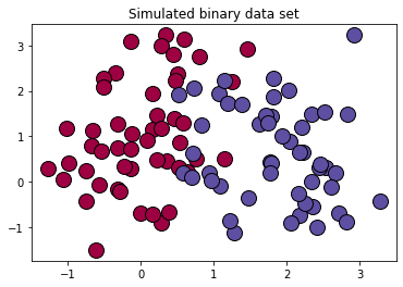

　　　　

复习

# 复习mylabel = label.reshape((-1,1))data = np.concatenate((x,mylabel),axis=1)print(data.shape)

结果：

(100, 3)

8 划分数据集

offset = int(x.shape[0]*0.7)x_train, y_train = x[:offset],label[:offset].reshape((-1,1)) x_test, y_test = x[offset:],label[offset:].reshape((-1,1)) print(x_train.shape)print(y_train.shape)print(x_test.shape)print(y_test.shape)

结果：

(70, 2)(70, 1)(30, 2)(30, 1)

9 训练

cost_list, params, grads = logistic_train(x_train, y_train, 0.01, 1000)print(params['b'])

结果：

epoch 0 cost 0.693147epoch 100 cost 0.568743epoch 200 cost 0.496925epoch 300 cost 0.449932epoch 400 cost 0.416618epoch 500 cost 0.391660epoch 600 cost 0.372186epoch 700 cost 0.356509epoch 800 cost 0.343574epoch 900 cost 0.332689-0.6646648941379839

10 准确率计算

from sklearn.metrics import accuracy_score,classification_reporty_pred = predict(x_test,params)print("y_pred = ",y_pred)print(y_pred)print(y_test.shape)print(accuracy_score(y_pred,y_test)) #不需要都是1维的，貌似会自动squeeze()print(classification_report(y_test,y_pred))

结果：

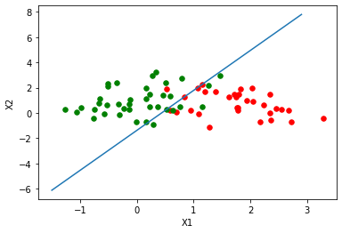
y_pred =  [0, 0, 1, 1, 1, 1, 0, 0, 0, 1, 1, 1, 0, 1, 1, 1, 1, 1, 1, 0, 0, 1, 1, 0, 1, 1, 0, 0, 1, 0][0, 0, 1, 1, 1, 1, 0, 0, 0, 1, 1, 1, 0, 1, 1, 1, 1, 1, 1, 0, 0, 1, 1, 0, 1, 1, 0, 0, 1, 0](30, 1)0.9333333333333333              precision    recall  f1-score   support           0       0.92      0.92      0.92        12           1       0.94      0.94      0.94        18    accuracy                           0.93        30   macro avg       0.93      0.93      0.93        30weighted avg       0.93      0.93      0.93        30

11 绘制逻辑回归决策边界

### 绘制逻辑回归决策边界def plot_logistic(X_train, y_train, params):    # 训练样本量    n = X_train.shape[0]    xcord1,ycord1,xcord2,ycord2 = [],[],[],[]    # 获取两类坐标点并存入列表    for i in range(n):        if y_train[i] == 1:            xcord1.append(X_train[i][0])            ycord1.append(X_train[i][1])        else:            xcord2.append(X_train[i][0])            ycord2.append(X_train[i][1])    fig = plt.figure()    ax = fig.add_subplot(111)    ax.scatter(xcord1,ycord1,s = 30,c = 'red')    ax.scatter(xcord2,ycord2,s = 30,c = 'green')    # 取值范围    x =np.arange(-1.5,3,0.1)    # 决策边界公式    y = (-params['b'] - params['W'][0] * x) / params['W'][1]    # 绘图    ax.plot(x, y)    plt.xlabel('X1')    plt.ylabel('X2')    plt.show()plot_logistic(x_train, y_train, params)

结果：

　　　　

11 sklearn实现

from sklearn.linear_model import LogisticRegressionclf = LogisticRegression(random_state=0).fit(x_train,y_train)y_pred = clf.predict(x_test)print(y_pred)accuracy_score(y_test,y_pred)

结果：

[0 0 1 1 1 1 0 0 0 1 1 1 0 1 1 0 0 1 1 0 0 1 1 0 1 1 0 0 1 0]0.9333333333333333