梅尔刻度(Mel scale)是一种由听众判断不同频率 音高(pitch)彼此相等的感知刻度,表示人耳对等距音高(pitch)变化的感知。mel 刻度和正常频率(Hz)之间的参考点是将1 kHz,且高于人耳听阈值40分贝以上的基音,定为1000 mel。在大约500 Hz以上,听者判断越来越大的音程(interval)产生相等的pitch增量,人耳每感觉到等量的音高变化,所需要的频率变化随频率增加而愈来愈大。
将频率$f$ (Hz)转换为梅尔$m$的公式是:
$$m=2595\log_{10}(1+\frac{f}{700})$$
def hz2mel(hz): """ Hz to Mels """ return 2595 * np.log10(1 + hz / 700.0)

mel与f(Hz)的对应关系


import numpy as npimport matplotlib.pyplot as pltfrom matplotlib.ticker import FuncFormatterdef hz2mel(hz): """ Hz to Mels """ return 2595 * np.log10(1 + hz / 700.0)if __name__ == "__main__": fs = 16000 hz = np.linspace(0, 8000, 8000) mel = hz2mel(hz) fig = plt.figure() ax = plt.plot(hz, mel, color="r") plt.xlabel("Hertz scale (Hz)", fontsize=12) # x轴的名字 plt.ylabel("mel scale", fontsize=12) plt.xticks(fontsize=10) # x轴的刻度 plt.yticks(fontsize=10) plt.xlim(0, 8000) # 坐标轴的范围 plt.ylim(0) def formatnum(x, pos): return '$%.1f$' % (x / 1000) formatter = FuncFormatter(formatnum) # plt.gca().xaxis.set_major_formatter(formatter) # plt.gca().yaxis.set_major_formatter(formatter) plt.grid(linestyle='--') plt.tight_layout() plt.show()
将梅尔$m$转换为频率$f$ (Hz)的公式是:
$$f=700e^{\frac{m}{2595}-1}$$
def mel2hz(mel): """ Mels to HZ """ return 700 * (10 ** (mel / 2595.0) - 1)
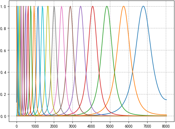
def mel_filterbanks(nfilt=20, nfft=512, samplerate=16000, lowfreq=0, highfreq=None): """计算一个Mel-filterbank (M,F) :param nfilt: filterbank中的滤波器数量 :param nfft: FFT size :param samplerate: 采样率 :param lowfreq: Mel-filter的最低频带边缘 :param highfreq: Mel-filter的最高频带边缘,默认samplerate/2 """ highfreq = highfreq or samplerate / 2 # 按梅尔均匀间隔计算 点 lowmel = hz2mel(lowfreq) highmel = hz2mel(highfreq) melpoints = np.linspace(lowmel, highmel, nfilt + 2) hz_points = mel2hz(melpoints) # 将mel频率再转到hz频率 # bin = samplerate/2 / NFFT/2=sample_rate/NFFT # 每个频点的频率数 # bins = hz_points/bin=hz_points*NFFT/ sample_rate # hz_points对应第几个fft频点 bin = np.floor((nfft + 1) * hz_points / samplerate) fbank = np.zeros([nfilt, int(nfft / 2 + 1)]) # (m,f) for i in range(0, nfilt): for j in range(int(bin[i]), int(bin[i + 1])): fbank[i, j] = (j - bin[i]) / (bin[i + 1] - bin[i]) for j in range(int(bin[i + 1]), int(bin[i + 2])): fbank[i, j] = (bin[i + 2] - j) / (bin[i + 2] - bin[i + 1]) # fbank -= (np.mean(fbank, axis=0) + 1e-8) return fbank


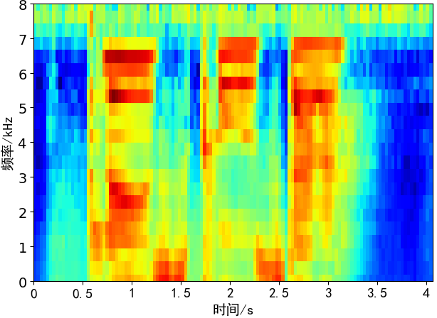
# -*- coding:utf-8 -*-# Author:凌逆战 | Never# Date: 2022/5/19"""1、提取Mel filterBank2、提取mel spectrum"""import librosaimport numpy as npimport matplotlib.pyplot as pltimport librosa.displayfrom matplotlib.ticker import FuncFormatterplt.rcParams['font.sans-serif'] = ['SimHei'] # 用来正常显示中文标签plt.rcParams['axes.unicode_minus'] = False # 用来正常显示符号def hz2mel(hz): """ Hz to Mels """ return 2595 * np.log10(1 + hz / 700.0)def mel2hz(mel): """ Mels to HZ """ return 700 * (10 ** (mel / 2595.0) - 1)def mel_filterbanks(nfilt=20, nfft=512, samplerate=16000, lowfreq=0, highfreq=None): """计算一个Mel-filterbank (M,F) :param nfilt: filterbank中的滤波器数量 :param nfft: FFT size :param samplerate: 采样率 :param lowfreq: Mel-filter的最低频带边缘 :param highfreq: Mel-filter的最高频带边缘,默认samplerate/2 """ highfreq = highfreq or samplerate / 2 # 按梅尔均匀间隔计算 点 lowmel = hz2mel(lowfreq) highmel = hz2mel(highfreq) melpoints = np.linspace(lowmel, highmel, nfilt + 2) hz_points = mel2hz(melpoints) # 将mel频率再转到hz频率 # bin = samplerate/2 / NFFT/2=sample_rate/NFFT # 每个频点的频率数 # bins = hz_points/bin=hz_points*NFFT/ sample_rate # hz_points对应第几个fft频点 bin = np.floor((nfft + 1) * hz_points / samplerate) fbank = np.zeros([nfilt, int(nfft / 2 + 1)]) # (m,f) for i in range(0, nfilt): for j in range(int(bin[i]), int(bin[i + 1])): fbank[i, j] = (j - bin[i]) / (bin[i + 1] - bin[i]) for j in range(int(bin[i + 1]), int(bin[i + 2])): fbank[i, j] = (bin[i + 2] - j) / (bin[i + 2] - bin[i + 1]) # fbank -= (np.mean(fbank, axis=0) + 1e-8) return fbankwav_path = "./p225_001.wav"fs = 16000NFFT = 512win_length = 512num_filter = 22low_freq_mel = 0high_freq_mel = hz2mel(fs // 2) # 求最高hz频率对应的mel频率mel_points = np.linspace(low_freq_mel, high_freq_mel, num_filter + 2) # 在mel频率上均分成42个点hz_points = mel2hz(mel_points) # 将mel频率再转到hz频率print(hz_points)# bin = sample_rate/2 / NFFT/2=sample_rate/NFFT # 每个频点的频率数# bins = hz_points/bin=hz_points*NFFT/ sample_rate # hz_points对应第几个fft频点bins = np.floor((NFFT + 1) * hz_points / fs)print(bins)# [ 0. 2. 5. 8. 12. 16. 20. 25. 31. 37. 44. 52. 61. 70.# 81. 93. 107. 122. 138. 157. 178. 201. 227. 256.]wav = librosa.load(wav_path, sr=fs)[0]S = librosa.stft(wav, n_fft=NFFT, hop_length=NFFT // 2, win_length=win_length, window="hann", center=False)mag = np.abs(S) # 幅度谱 (257, 127) librosa.magphase()filterbanks = mel_filterbanks(nfilt=num_filter, nfft=NFFT, samplerate=fs, lowfreq=0, highfreq=fs // 2)# ================ 画三角滤波器 ===========================FFT_len = NFFT // 2 + 1fs_bin = fs // 2 / (NFFT // 2) # 一个频点多少Hzx = np.linspace(0, FFT_len, FFT_len)plt.plot(x * fs_bin, filterbanks.T)plt.xlim(0) # 坐标轴的范围plt.ylim(0, 1)plt.tight_layout()plt.grid(linestyle='--')plt.show()filter_banks = np.dot(filterbanks, mag) # (M,F)*(F,T)=(M,T)filter_banks = 20 * np.log10(filter_banks) # dB# ================ 绘制语谱图 ==========================# 绘制 频谱图 方法1plt.imshow(filter_banks, cmap="jet", aspect='auto')ax = plt.gca() # 获取其中某个坐标系ax.invert_yaxis() # 将y轴反转plt.tight_layout()plt.show()# 绘制 频谱图 方法2plt.figure()librosa.display.specshow(filter_banks, sr=fs, x_axis='time', y_axis='linear', cmap="jet")plt.xlabel('时间/s', fontsize=14)plt.ylabel('频率/kHz', fontsize=14)plt.xticks(fontsize=14)plt.yticks(fontsize=14)def formatnum(x, pos): return '$%d$' % (x / 1000)formatter = FuncFormatter(formatnum)plt.gca().yaxis.set_major_formatter(formatter)plt.tight_layout()plt.show()
另外Librosa写好了完整的提取mel频谱和MFCC的API:
mel_spec = librosa.feature.melspectrogram(y=y, sr=sr, n_mels=128, fmax=8000)mfccs = librosa.feature.mfcc(y=y, sr=sr, n_mfcc=40)巴克刻度(Bark scale)是于1961年由德国声学家Eberhard Zwicker提出的一种心理声学的尺度。它以Heinrich Barkhausen的名字命名,他提出了响度的第一个主观测量。[1]该术语的一个定义是“……等距离对应于感知上等距离的频率刻度”。高于约 500 Hz 时,此刻度或多或少等于对数频率轴。低于 500 Hz 时,Bark 标度变为越来越线性”。bark 刻度的范围是从1到24,并且它们与听觉的临界频带相对应。
频率f (Hz) 转换为 Bark:
$$\text { Bark }=13 \arctan (0.00076 f)+3.5 \arctan ((\frac{f}{7500})^{2})$$
Traunmüller, 1990 提出的新的Bark scale公式:
$$\operatorname{Bark}=\frac{26.81f}{1960+f}-0.53$$
反转:$f=\frac{1960((\operatorname{Bark}+0.53)-1)}{26.81}$
临界带宽(Hz):$B_c=\frac{52548}{\operatorname{Bark}^2-52.56\operatorname{Bark}+690.39}$
Wang, Sekey & Gersho, 1992 提出了新的Bark scale公式:
$$\text { Bark }=6 \sinh ^{-1}(\frac{f}{600})$$
def hz2bark_1961(Hz): return 13.0 * np.arctan(0.00076 * Hz) + 3.5 * np.arctan((Hz / 7500.0) ** 2)def hz2bark_1990(Hz): bark_scale = (26.81 * Hz) / (1960 + Hz) - 0.5 return bark_scaledef hz2bark_1992(Hz): return 6 * np.arcsinh(Hz / 600)

import numpy as npimport matplotlib.pyplot as pltfrom matplotlib.ticker import FuncFormatterdef hz2bark_1961(Hz): return 13.0 * np.arctan(0.00076 * Hz) + 3.5 * np.arctan((Hz / 7500.0) ** 2)def hz2bark_1990(Hz): bark_scale = (26.81 * Hz) / (1960 + Hz) - 0.5 return bark_scaledef hz2bark_1992(Hz): return 6 * np.arcsinh(Hz / 600)if __name__ == "__main__": fs = 16000 hz = np.linspace(0, fs // 2, fs // 2) bark_1961 = hz2bark_1961(hz) bark_1990 = hz2bark_1990(hz) bark_1992 = hz2bark_1992(hz) plt.plot(hz, bark_1961, label="bark_1961") plt.plot(hz, bark_1990, label="bark_1990") plt.plot(hz, bark_1992, label="bark_1992") plt.legend() # 显示图例 plt.xlabel("Hertz scale (Hz)", fontsize=12) # x轴的名字 plt.ylabel("Bark scale", fontsize=12) plt.xticks(fontsize=10) # x轴的刻度 plt.yticks(fontsize=10) plt.xlim(0, fs // 2) # 坐标轴的范围 plt.ylim(0) def formatnum(x, pos): return '$%.1f$' % (x / 1000) formatter = FuncFormatter(formatnum) # plt.gca().xaxis.set_major_formatter(formatter) # plt.gca().yaxis.set_major_formatter(formatter) plt.grid(linestyle='--') plt.tight_layout() plt.show()


import numpy as npimport librosaimport librosa.displayimport matplotlib.pyplot as pltfrom matplotlib.ticker import FuncFormatterplt.rcParams['font.sans-serif'] = ['SimHei'] # 用来正常显示中文标签plt.rcParams['axes.unicode_minus'] = False # 用来正常显示符号def hz2bark(f): """ Hz to bark频率 (Wang, Sekey & Gersho, 1992.) """ return 6. * np.arcsinh(f / 600.)def bark2hz(fb): """ Bark频率 to Hz """ return 600. * np.sinh(fb / 6.)def fft2hz(fft, fs=16000, nfft=512): """ FFT频点 to Hz """ return (fft * fs) / (nfft + 1)def hz2fft(fb, fs=16000, nfft=512): """ Bark频率 to FFT频点 """ return (nfft + 1) * fb / fsdef fft2bark(fft, fs=16000, nfft=512): """ FFT频点 to Bark频率 """ return hz2bark((fft * fs) / (nfft + 1))def bark2fft(fb, fs=16000, nfft=512): """ Bark频率 to FFT频点 """ # bin = sample_rate/2 / nfft/2=sample_rate/nfft # 每个频点的频率数 # bins = hz_points/bin=hz_points*nfft/ sample_rate # hz_points对应第几个fft频点 return (nfft + 1) * bark2hz(fb) / fsdef Fm(fb, fc): """ 计算一个特定的中心频率的Bark filter :param fb: frequency in Bark. :param fc: center frequency in Bark. :return: 相关的Bark filter 值/幅度 """ if fc - 2.5 <= fb <= fc - 0.5: return 10 ** (2.5 * (fb - fc + 0.5)) elif fc - 0.5 < fb < fc + 0.5: return 1 elif fc + 0.5 <= fb <= fc + 1.3: return 10 ** (-2.5 * (fb - fc - 0.5)) else: return 0def bark_filter_banks(nfilts=20, nfft=512, fs=16000, low_freq=0, high_freq=None, scale="constant"): """ 计算Bark-filterbanks,(B,F) :param nfilts: 滤波器组中滤波器的数量 (Default 20) :param nfft: FFT size.(Default is 512) :param fs: 采样率,(Default 16000 Hz) :param low_freq: MEL滤波器的最低带边。(Default 0 Hz) :param high_freq: MEL滤波器的最高带边。(Default samplerate/2) :param scale (str): 选择Max bins 幅度 "ascend"(上升),"descend"(下降)或 "constant"(恒定)(=1)。默认是"constant" :return:一个大小为(nfilts, nfft/2 + 1)的numpy数组,包含滤波器组。 """ # init freqs high_freq = high_freq or fs / 2 low_freq = low_freq or 0 # 按Bark scale 均匀间隔计算点数(点数以Bark为单位) low_bark = hz2bark(low_freq) high_bark = hz2bark(high_freq) bark_points = np.linspace(low_bark, high_bark, nfilts + 4) bins = np.floor(bark2fft(bark_points)) # Bark Scale等分布对应的 FFT bin number # [ 0. 2. 5. 7. 10. 13. 16. 20. 24. 28. 33. 38. 44. 51. # 59. 67. 77. 88. 101. 115. 132. 151. 172. 197. 224. 256.] fbank = np.zeros([nfilts, nfft // 2 + 1]) # init scaler if scale == "descendant" or scale == "constant": c = 1 else: c = 0 for i in range(0, nfilts): # --> B # compute scaler if scale == "descendant": c -= 1 / nfilts c = c * (c > 0) + 0 * (c < 0) elif scale == "ascendant": c += 1 / nfilts c = c * (c < 1) + 1 * (c > 1) for j in range(int(bins[i]), int(bins[i + 4])): # --> F fc = bark_points[i+2] # 中心频率 fb = fft2bark(j) # Bark 频率 fbank[i, j] = c * Fm(fb, fc) return np.abs(fbank)if __name__ == "__main__": nfilts = 22 NFFT = 512 fs = 16000 wav = librosa.load("p225_001.wav",sr=fs)[0] S = librosa.stft(wav, n_fft=NFFT, hop_length=NFFT // 2, win_length=NFFT, window="hann", center=False) mag = np.abs(S) # 幅度谱 (257, 127) librosa.magphase() filterbanks = bark_filter_banks(nfilts=nfilts, nfft=NFFT, fs=fs, low_freq=0, high_freq=None, scale="constant") # ================ 画三角滤波器 =========================== FFT_len = NFFT // 2 + 1 fs_bin = fs // 2 / (NFFT // 2) # 一个频点多少Hz x = np.linspace(0, FFT_len, FFT_len) plt.plot(x * fs_bin, filterbanks.T) # plt.xlim(0) # 坐标轴的范围 # plt.ylim(0, 1) plt.tight_layout() plt.grid(linestyle='--') plt.show() filter_banks = np.dot(filterbanks, mag) # (M,F)*(F,T)=(M,T) filter_banks = 20 * np.log10(filter_banks) # dB # ================ 绘制语谱图 ========================== plt.figure() librosa.display.specshow(filter_banks, sr=fs, x_axis='time', y_axis='linear', cmap="jet") plt.xlabel('时间/s', fontsize=14) plt.ylabel('频率/kHz', fontsize=14) plt.xticks(fontsize=14) plt.yticks(fontsize=14) def formatnum(x, pos): return '$%d$' % (x / 1000) formatter = FuncFormatter(formatnum) plt.gca().yaxis.set_major_formatter(formatter) plt.tight_layout() plt.show()
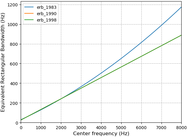
等效矩形带宽(Equivalent Rectangular Bandwidth,ERB)是用于心理声学(研究人对声音(包括言语和音乐)的生理和心理反应的科学)的一种量度方法,它给出了一个近似于 人耳听觉的对带宽的过滤方法,使用不现实但方便的简化方法将滤波器建模为矩形带通滤波器或带阻滤波器。
Moore 和 Glasberg在1983 年,对于中等的声强和年轻的听者,人的听觉滤波器的带宽可以通过以下的多项式方程式近似:
$$公式1:\operatorname{ERB}(f)=6.23 \cdot f^{2}+93.39 \cdot f+28.52$$
其中$f$为滤波器的中心频率(kHz),$ERB(f)$为滤波器的带宽(Hz)。这个近似值是基于一些出版的同时掩蔽(Simultaneous masking)实验的结果。这个近似对于从0.1到6.5 kHz的范围是有效的。
它们也在1990年发表了另一(线性)近似:
$$公式2:\operatorname{ERB}(f)=24.7 \cdot(4.37 \cdot f+1)$$
其中$f$的单位是 kHz,$ERB(f)$的单位是 Hz。这个近似值适用于中等声级和0.1 到 10 kHz 之间的频率值。
def hz2erb_1983(f): """ 中心频率f(Hz) f to ERB(Hz) """ f = f / 1000.0 return (6.23 * (f ** 2)) + (93.39 * f) + 28.52def hz2erb_1990(f): """ 中心频率f(Hz) f to ERB(Hz) """ f = f / 1000.0 return 24.7 * (4.37 * f + 1.0)def hz2erb_1998(f): """ 中心频率f(Hz) f to ERB(Hz) hz2erb_1990 和 hz2erb_1990_2 的曲线几乎一模一样 M. Slaney, Auditory Toolbox, Version 2, Technical Report No: 1998-010, Internal Research Corporation, 1998 http://cobweb.ecn.purdue.edu/~malcolm/interval/1998-010/ """ return 24.7 + (f / 9.26449)
给定频率$f$可以求得 等效矩形带宽的数量(Number of ERB, ERBs)。ERBs可以通过求解以下微分方程组来构建量表:
$$公式3:\left\{\begin{array}{l}
\operatorname{ERBs}(0)=0 \\
\frac{d f}{d \operatorname{ERBs}(f)}=\operatorname{ERB}(f)
\end{array}\right.$$
使用ERB(f)公式1可求得ERBs:
$$ \operatorname{ERBs}(f)=11.17 \cdot \ln \left(\frac{f+0.312}{f+14.675}\right)+43.0$$
其中$f$以 kHz 为单位。
用于MATLAB的 VOICEBOX 语音处理工具箱将转换及其逆实现为:
$$\operatorname{ERBs}(f)=11.17268 \cdot \ln \left(1+\frac{46.06538 \cdot f}{f+14678.49}\right)$$
$$f=\frac{676170.4}{47.06538-e^{0.08950404 \cdot \operatorname{ERBs}(f)}}-14678.49$$
其中$f$以Hz为单位。
def erb_matlab_voicebox(f: float) -> float: cuotient = (46.06538 * f) / float(f + 14678.49) return 11.17268 * math.log(1 + cuotient)def ierb_matlab_voicebox(erbf: float) -> float: denom = 47.06538 - math.exp(0.08950404 - erbf) return (676170.4 / float(denom)) - 14678.49
使用ERB(f)公式2可得:
$$\operatorname{ERBS}(f)=21.4 \cdot \log _{10}(1+ \frac{4.37\cdot f}{1000})$$
其中$f$以赫兹为单位。
使用ERB的线性滤波器组
# -*- coding:utf-8 -*-# Author:凌逆战 | Never.Ling# Date: 2022/5/28"""基于Josh McDermott的Matlab滤波器组代码:https://github.com/wil-j-wil/py_bankhttps://github.com/flavioeverardo/erb_bands"""import numpy as npimport librosaimport librosa.displayimport matplotlib.pyplot as pltfrom matplotlib.ticker import FuncFormatterplt.rcParams['font.sans-serif'] = ['SimHei'] # 用来正常显示中文标签plt.rcParams['axes.unicode_minus'] = False # 用来正常显示符号class EquivalentRectangularBandwidth(): def __init__(self, nfreqs, sample_rate, total_erb_bands, low_freq, max_freq): if low_freq == None: low_freq = 20 if max_freq == None: max_freq = sample_rate // 2 freqs = np.linspace(0, max_freq, nfreqs) # 每个STFT频点对应多少Hz self.EarQ = 9.265 # _ERB_Q self.minBW = 24.7 # minBW # 在ERB刻度上建立均匀间隔 erb_low = self.freq2erb(low_freq) # 最低 截止频率 erb_high = self.freq2erb(max_freq) # 最高 截止频率 # 在ERB频率上均分为(total_erb_bands + )2个 频带 erb_lims = np.linspace(erb_low, erb_high, total_erb_bands + 2) cutoffs = self.erb2freq(erb_lims) # 将 ERB频率再转到 hz频率, 在线性频率Hz上找到ERB截止频率对应的频率 # self.nfreqs F # self.freqs # 每个STFT频点对应多少Hz self.filters = self.get_bands(total_erb_bands, nfreqs, freqs, cutoffs) def freq2erb(self, frequency): """ [Hohmann2002] Equation 16""" return self.EarQ * np.log(1 + frequency / (self.minBW * self.EarQ)) def erb2freq(self, erb): """ [Hohmann2002] Equation 17""" return (np.exp(erb / self.EarQ) - 1) * self.minBW * self.EarQ def get_bands(self, total_erb_bands, nfreqs, freqs, cutoffs): """ 获取erb bands、索引、带宽和滤波器形状 :param erb_bands_num: ERB 频带数 :param nfreqs: 频点数 F :param freqs: 每个STFT频点对应多少Hz :param cutoffs: 中心频率 Hz :param erb_points: ERB频带界限 列表 :return: """ cos_filts = np.zeros([nfreqs, total_erb_bands]) # (F, ERB) for i in range(total_erb_bands): lower_cutoff = cutoffs[i] # 上限截止频率 Hz higher_cutoff = cutoffs[i + 2] # 下限截止频率 Hz, 相邻filters重叠50% lower_index = np.min(np.where(freqs > lower_cutoff)) # 下限截止频率对应的Hz索引 Hz。np.where 返回满足条件的索引 higher_index = np.max(np.where(freqs < higher_cutoff)) # 上限截止频率对应的Hz索引 avg = (self.freq2erb(lower_cutoff) + self.freq2erb(higher_cutoff)) / 2 rnge = self.freq2erb(higher_cutoff) - self.freq2erb(lower_cutoff) cos_filts[lower_index:higher_index + 1, i] = np.cos( (self.freq2erb(freqs[lower_index:higher_index + 1]) - avg) / rnge * np.pi) # 减均值,除方差 # 加入低通和高通,得到完美的重构 filters = np.zeros([nfreqs, total_erb_bands + 2]) # (F, ERB) filters[:, 1:total_erb_bands + 1] = cos_filts # 低通滤波器上升到第一个余cos filter的峰值 higher_index = np.max(np.where(freqs < cutoffs[1])) # 上限截止频率对应的Hz索引 filters[:higher_index + 1, 0] = np.sqrt(1 - np.power(filters[:higher_index + 1, 1], 2)) # 高通滤波器下降到最后一个cos filter的峰值 lower_index = np.min(np.where(freqs > cutoffs[total_erb_bands])) filters[lower_index:nfreqs, total_erb_bands + 1] = np.sqrt( 1 - np.power(filters[lower_index:nfreqs, total_erb_bands], 2)) return cos_filtsif __name__ == "__main__": fs = 16000 NFFT = 512 # 信号长度 ERB_num = 20 low_lim = 20 # 最低滤波器中心频率 high_lim = fs / 2 # 最高滤波器中心频率 freq_num = NFFT // 2 + 1 fs_bin = fs // 2 / (NFFT // 2) # 一个频点多少Hz x = np.linspace(0, freq_num, freq_num) # ================ 画三角滤波器 =========================== ERB = EquivalentRectangularBandwidth(freq_num, fs, ERB_num, low_lim, high_lim) filterbanks = ERB.filters.T # (257, 20) plt.plot(x * fs_bin, filterbanks.T) # plt.xlim(0) # 坐标轴的范围 # plt.ylim(0, 1) plt.tight_layout() plt.grid(linestyle='--') plt.show() # ================ 绘制语谱图 ========================== wav = librosa.load("p225_001.wav", sr=fs)[0] S = librosa.stft(wav, n_fft=NFFT, hop_length=NFFT // 2, win_length=NFFT, window="hann", center=False) mag = np.abs(S) # 幅度谱 (257, 127) librosa.magphase() filter_banks = np.dot(filterbanks, mag) # (M,F)*(F,T)=(M,T) filter_banks = 20 * np.log10(filter_banks) # dB plt.figure() librosa.display.specshow(filter_banks, sr=fs, x_axis='time', y_axis='linear', cmap="jet") plt.xlabel('时间/s', fontsize=14) plt.ylabel('频率/kHz', fontsize=14) plt.xticks(fontsize=14) plt.yticks(fontsize=14) def formatnum(x, pos): return '$%d$' % (x / 1000) formatter = FuncFormatter(formatnum) plt.gca().yaxis.set_major_formatter(formatter) plt.tight_layout() plt.show()


外界语音信号进入耳蜗的基底膜后,将依据频率进行分解并产生行波震动,从而刺激听觉感受细胞。GammaTone 滤波器是一组用来模拟耳蜗频率分解特点的滤波器模型,由脉冲响应描述的线性滤波器,脉冲响应是gamma 分布和正弦(sin)音调的乘积。它是听觉系统中一种广泛使用的听觉滤波器模型。
历史
一般认为外周听觉系统的频率分析方式可以通过一组带通滤波器来进行一定程度的模拟,人们为此也提出了各种各样的滤波器组,如 roex 滤波器(Patterson and Moore 1986)。
在神经科学上有一种叫做反向相关性 “reverse correlation”(de Boer and Kuyper 1968)的计算方式,通过计算初级听觉神经纤维对于白噪声刺激的响应以及相关程度,即听觉神经元发放动作电位前的平均叠加信号,从而直接从生理状态上估计听觉滤波器的形状。这个滤波器是在外周听觉神经发放动作电位前生效的,因此得名为“revcor function”,可以作为一定限度下对外周听觉滤波器冲激响应的估计,也就是耳蜗等对音频信号的前置带通滤波。
1972年Johannesma提出了 gammatone 滤波器用来逼近recvor function:
$$时域表达式:g(t)=a t^{n-1} e^{-2 \pi b t} \cos (2 \pi f_c t+\phi_0)$$
其中$f_c(Hz)$是中心频率(center frequency),$\phi_0$是初始相位(phase),$a$是幅度(amplitude),$n$是滤波器的阶数(order),越大则偏度越低,滤波器越“瘦高”,$b(Hz)$是滤波器的3dB 带宽(bandwidth),$t(s)$是时间。

这个时域脉冲响应是一个正弦曲线(pure tone),其幅度包络是一个缩放的gamma分布函数。
我们可以通过时域表达式生成一组gammatone滤波器组 和 gammatone滤波器组特征。
# -*- coding:utf-8 -*-# Author:凌逆战 | Never.Ling# Date: 2022/5/24"""时域滤波器组 FFT 转频域滤波器组 与语音频谱相乘参考:https://github.com/TAriasVergara/Acoustic_features"""import librosaimport librosa.displayimport numpy as npfrom scipy.fftpack import dctimport matplotlib.pyplot as pltfrom matplotlib.ticker import FuncFormatterplt.rcParams['font.sans-serif'] = ['SimHei'] # 用来正常显示中文标签plt.rcParams['axes.unicode_minus'] = False # 用来正常显示符号def erb_space(low_freq=50, high_freq=8000, n=64): """ 计算中心频率(ERB scale) :param min_freq: 中心频率域的最小频率。 :param max_freq: 中心频率域的最大频率。 :param nfilts: 滤波器的个数,即等于计算中心频率的个数。 :return: 一组中心频率 """ ear_q = 9.26449 min_bw = 24.7 cf_array = -(ear_q * min_bw) + np.exp( np.linspace(1, n, n) * (-np.log(high_freq + ear_q * min_bw) + np.log(low_freq + ear_q * min_bw)) / n) \ * (high_freq + ear_q * min_bw) return cf_arraydef gammatone_impulse_response(samplerate_hz, length_in_samples, center_freq_hz, p): """ gammatone滤波器的时域公式 :param samplerate_hz: 采样率 :param length_in_samples: 信号长度 :param center_freq_hz: 中心频率 :param p: 滤波器阶数 :return: gammatone 脉冲响应 """ # 生成一个gammatone filter (1990 Glasberg&Moore parametrized) erb = 24.7 + (center_freq_hz / 9.26449) # equivalent rectangular bandwidth. # 中心频率 an = (np.pi * np.math.factorial(2 * p - 2) * np.power(2, float(-(2 * p - 2)))) / np.square(np.math.factorial(p - 1)) b = erb / an # 带宽 a = 1 # 幅度(amplitude). 这在后面的归一化过程中有所不同。 t = np.linspace(1. / samplerate_hz, length_in_samples / samplerate_hz, length_in_samples) gammatone_ir = a * np.power(t, p - 1) * np.exp(-2 * np.pi * b * t) * np.cos(2 * np.pi * center_freq_hz * t) return gammatone_irdef generate_filterbank(fs, fmax, L, N, p=4): """ L: 在样本中测量的信号的大小 N: 滤波器数量 p: Gammatone脉冲响应的阶数 """ # 中心频率 if fs == 8000: fmax = 4000 center_freqs = erb_space(50, fmax, N) # 中心频率列表 center_freqs = np.flip(center_freqs) # 反转数组 n_center_freqs = len(center_freqs) # 中心频率的数量 filterbank = np.zeros((N, L)) # 为每个中心频率生成 滤波器 for i in range(n_center_freqs): # aa = gammatone_impulse_response(fs, L, center_freqs[i], p) filterbank[i, :] = gammatone_impulse_response(fs, L, center_freqs[i], p) return filterbankdef gfcc(cochleagram, numcep=13): feat = dct(cochleagram, type=2, axis=1, norm='ortho')[:, :numcep] # feat-= (np.mean(feat, axis=0) + 1e-8)#Cepstral mean substration return featdef cochleagram(sig_spec, filterbank, nfft): """ :param sig_spec: 语音频谱 :param filterbank: 时域滤波器组 :param nfft: fft_size :return: """ filterbank = powerspec(filterbank, nfft) # 时域滤波器组经过FFT变换 filterbank /= np.max(filterbank, axis=-1)[:, None] # Normalize filters cochlea_spec = np.dot(sig_spec, filterbank.T) # 矩阵相乘 cochlea_spec = np.where(cochlea_spec == 0.0, np.finfo(float).eps, cochlea_spec) # 把0变成一个很小的数 # cochlea_spec= np.log(cochlea_spec)-np.mean(np.log(cochlea_spec),axis=0) cochlea_spec = np.log(cochlea_spec) return cochlea_spec, filterbankdef powerspec(X, nfft): # Fourier transform # Y = np.fft.rfft(X, n=n_padded) Y = np.fft.fft(X, n=nfft) Y = np.absolute(Y) # non-redundant part m = int(nfft / 2) + 1 Y = Y[:, :m] return np.abs(Y) ** 2if __name__ == "__main__": nfilts = 22 NFFT = 512 fs = 16000 Order = 4 FFT_len = NFFT // 2 + 1 fs_bin = fs // 2 / (NFFT // 2) # 一个频点多少Hz x = np.linspace(0, FFT_len, FFT_len) # ================ 画三角滤波器 =========================== # gammatone_impulse_response = gammatone_impulse_response(fs/2, 512, 200, Order) # gammatone冲击响应 generate_filterbank = generate_filterbank(fs, fs // 2, FFT_len, nfilts, Order) filterbanks = powerspec(generate_filterbank, NFFT) # 时域滤波器组经过FFT变换 filterbanks /= np.max(filterbanks, axis=-1)[:, None] # Normalize filters print(generate_filterbank.shape) # (22, 257) # plt.plot(filterbanks.T) plt.plot(x * fs_bin, filterbanks.T) # plt.xlim(0) # 坐标轴的范围 # plt.ylim(0, 1) plt.tight_layout() plt.grid(linestyle='--') plt.show() # ================ 绘制语谱图 ========================== wav = librosa.load("p225_001.wav", sr=fs)[0] S = librosa.stft(wav, n_fft=NFFT, hop_length=NFFT // 2, win_length=NFFT, window="hann", center=False) mag = np.abs(S) # 幅度谱 (257, 127) librosa.magphase() filter_banks = np.dot(filterbanks, mag) # (M,F)*(F,T)=(M,T) filter_banks = 20 * np.log10(filter_banks) # dB plt.figure() librosa.display.specshow(filter_banks, sr=fs, x_axis='time', y_axis='linear', cmap="jet") plt.xlabel('时间/s', fontsize=14) plt.ylabel('频率/kHz', fontsize=14) plt.xticks(fontsize=14) plt.yticks(fontsize=14) def formatnum(x, pos): return '$%d$' % (x / 1000) formatter = FuncFormatter(formatnum) plt.gca().yaxis.set_major_formatter(formatter) plt.tight_layout() plt.show()


可以看到低频段分得很细,高频段分得很粗,和人耳听觉特性较为符合。
$$频域表达式:\begin{aligned}
H(f)=& a[R(f) \otimes S(f)] \\
=& \frac{a}{2}(n-1) !(2 \pi b)^{-n}\left\{e^{i \phi_0}\left[1+\frac{i(f-f_c)}{b} \right]^{-n}+e^{-i \phi_0}\left[1+\frac{i(f+f_c)}{b}\right]^{-n}\right\}
\end{aligned}$$
频率表达式中$R(f)$是 指数+阶跃函数的傅里叶变换,阶跃函数用来区别 t>0 和 t<0。$S(f)$是频率为$f_0$的余弦的傅里叶变换。可以看到是一个中心频率在$f_c$、 在两侧按照e指数衰减的滤波器。通过上述表达式可以生成一组滤波器,求Gammatone滤波器组特征 只需要将Gammatone滤波器组与语音幅度谱相乘即可得到Gammatone滤波器组特征。
# -*- coding:utf-8 -*-# Author:凌逆战 | Never# Date: 2022/5/24"""Gammatone-filter-banks implementationbased on https://github.com/mcusi/gammatonegram/"""import librosaimport librosa.displayimport numpy as npfrom matplotlib import pyplot as pltfrom matplotlib.ticker import FuncFormatterplt.rcParams['font.sans-serif'] = ['SimHei'] # 用来正常显示中文标签plt.rcParams['axes.unicode_minus'] = False # 用来正常显示符号# Slaney's ERB Filter constantsEarQ = 9.26449minBW = 24.7def generate_center_frequencies(min_freq, max_freq, filter_nums): """ 计算中心频率(ERB scale) :param min_freq: 中心频率域的最小频率。 :param max_freq: 中心频率域的最大频率。 :param filter_nums: 滤波器的个数,即等于计算中心频率的个数。 :return: 一组中心频率 """ # init vars n = np.linspace(1, filter_nums, filter_nums) c = EarQ * minBW # 计算中心频率 cfreqs = (max_freq + c) * np.exp((n / filter_nums) * np.log( (min_freq + c) / (max_freq + c))) - c return cfreqsdef compute_gain(fcs, B, wT, T): """ 为了 阶数 计算增益和矩阵化计算 :param fcs: 中心频率 :param B: 滤波器的带宽 :param wT: 对应于用于频域计算的 w * T = 2 * pi * freq * T :param T: 周期(单位秒s),1/fs :return: Gain: 表示filter gains 的2d numpy数组 A: 用于最终计算的二维数组 """ # 为了简化 预先计算 K = np.exp(B * T) Cos = np.cos(2 * fcs * np.pi * T) Sin = np.sin(2 * fcs * np.pi * T) Smax = np.sqrt(3 + 2 ** (3 / 2)) Smin = np.sqrt(3 - 2 ** (3 / 2)) # 定义A矩阵的行 A11 = (Cos + Smax * Sin) / K A12 = (Cos - Smax * Sin) / K A13 = (Cos + Smin * Sin) / K A14 = (Cos - Smin * Sin) / K # 计算增益 (vectorized) A = np.array([A11, A12, A13, A14]) Kj = np.exp(1j * wT) Kjmat = np.array([Kj, Kj, Kj, Kj]).T G = 2 * T * Kjmat * (A.T - Kjmat) Coe = -2 / K ** 2 - 2 * Kj ** 2 + 2 * (1 + Kj ** 2) / K Gain = np.abs(G[:, 0] * G[:, 1] * G[:, 2] * G[:, 3] * Coe ** -4) return A, Gaindef gammatone_filter_banks(nfilts=22, nfft=512, fs=16000, low_freq=None, high_freq=None, scale="contsant", order=4): """ 计算Gammatone-filterbanks, (G,F) :param nfilts: filterbank中滤波器的数量 (Default 22) :param nfft: FFT size (Default is 512) :param fs: 采样率 (Default 16000 Hz) :param low_freq: 最低频带 (Default 0 Hz) :param high_freq: 最高频带 (Default samplerate/2) :param scale: 选择Max bins 幅度 "ascend"(上升),"descend"(下降)或 "constant"(恒定)(=1)。默认是"constant" :param order: 滤波器阶数 :return: 一个大小为(nfilts, nfft/2 + 1)的numpy数组,包含滤波器组。 """ # init freqs high_freq = high_freq or fs / 2 low_freq = low_freq or 0 # define custom difference func def Dif(u, a): return u - a.reshape(nfilts, 1) # init vars fbank = np.zeros([nfilts, nfft]) width = 1.0 maxlen = nfft // 2 + 1 T = 1 / fs n = 4 u = np.exp(1j * 2 * np.pi * np.array(range(nfft // 2 + 1)) / nfft) idx = range(nfft // 2 + 1) fcs = generate_center_frequencies(low_freq, high_freq, nfilts) # 计算中心频率,转换到ERB scale ERB = width * ((fcs / EarQ) ** order + minBW ** order) ** (1 / order) # 计算带宽 B = 1.019 * 2 * np.pi * ERB # compute input vars wT = 2 * fcs * np.pi * T pole = np.exp(1j * wT) / np.exp(B * T) # compute gain and A matrix A, Gain = compute_gain(fcs, B, wT, T) # compute fbank fbank[:, idx] = ( (T ** 4 / Gain.reshape(nfilts, 1)) * np.abs(Dif(u, A[0]) * Dif(u, A[1]) * Dif(u, A[2]) * Dif(u, A[3])) * np.abs(Dif(u, pole) * Dif(u, pole.conj())) ** (-n)) # 确保所有filters的最大值为1.0 try: fbs = np.array([f / np.max(f) for f in fbank[:, range(maxlen)]]) except BaseException: fbs = fbank[:, idx] # compute scaler if scale == "ascendant": c = [ 0, ] for i in range(1, nfilts): x = c[i - 1] + 1 / nfilts c.append(x * (x < 1) + 1 * (x > 1)) elif scale == "descendant": c = [ 1, ] for i in range(1, nfilts): x = c[i - 1] - 1 / nfilts c.append(x * (x > 0) + 0 * (x < 0)) else: c = [1 for i in range(nfilts)] # apply scaler c = np.array(c).reshape(nfilts, 1) fbs = c * np.abs(fbs) return fbsif __name__ == "__main__": nfilts = 22 NFFT = 512 fs = 16000 FFT_len = NFFT // 2 + 1 fs_bin = fs // 2 / (NFFT // 2) # 一个频点多少Hz x = np.linspace(0, FFT_len, FFT_len) # ================ 画三角滤波器 =========================== filterbanks = gammatone_filter_banks(nfilts=22, nfft=512, fs=16000, low_freq=None, high_freq=None, scale="contsant", order=4) print(filterbanks.shape) # (22, 257) plt.plot(x * fs_bin, filterbanks.T) # plt.xlim(0) # 坐标轴的范围 # plt.ylim(0, 1) plt.tight_layout() plt.grid(linestyle='--') plt.show() # ================ 绘制语谱图 ========================== wav = librosa.load("p225_001.wav", sr=fs)[0] S = librosa.stft(wav, n_fft=NFFT, hop_length=NFFT // 2, win_length=NFFT, window="hann", center=False) mag = np.abs(S) # 幅度谱 (257, 127) librosa.magphase() filter_banks = np.dot(filterbanks, mag) # (M,F)*(F,T)=(M,T) filter_banks = 20 * np.log10(filter_banks) # dB plt.figure() librosa.display.specshow(filter_banks, sr=fs, x_axis='time', y_axis='linear', cmap="jet") plt.xlabel('时间/s', fontsize=14) plt.ylabel('频率/kHz', fontsize=14) plt.xticks(fontsize=14) plt.yticks(fontsize=14) def formatnum(x, pos): return '$%d$' % (x / 1000) formatter = FuncFormatter(formatnum) plt.gca().yaxis.set_major_formatter(formatter) plt.tight_layout() plt.show()
1988年Holdsworth 等人进一步阐明了GTF的各种特性,而且提供了一个数字IIR滤波器设计方案。这个技术使得GTF能够比FIR更加容易且高效地实现,为后续出现一些重要的实际应用做了铺垫。听觉滤波的gammatone模型的变化和改进包括复数gammatone滤波器、gammachirp滤波器、全极点(all-pole)和一零(one-zero) gammatone滤波器、双边(two-sided)gammatone滤波器和滤波器级联(filter-cascade)模型,以及各种level相关和这些的动态非线性版本。
【博客】Auditory scales of frequency representation
【百度百科】心理声学
【维基百科】Bark scale
【维基百科】Mel scale
【维基百科】Equivalent rectangular bandwidth
【维基百科】Gammatone filter(包含了C \ C++ \ mathematica \ matlab的代码实现)
【博客】Equivalent Rectangular Bandwidth
【CSDN】GammaTone 滤波器详解
【python库】PyFilterbank
【代码】Brookes, Mike (22 December 2012). "frq2erb". VOICEBOX: Speech Processing Toolbox for MATLAB. Department of Electrical & Electronic Engineering, Imperial College, UK. Retrieved 20 January 2013.
【代码】Brookes, Mike (22 December 2012). "erb2frq". VOICEBOX: Speech Processing Toolbox for MATLAB. Department of Electrical & Electronic Engineering, Imperial College, UK. Retrieved 20 January 2013.
【论文】Smith, Julius O.; Abel, Jonathan S. (10 May 2007). "Equivalent Rectangular Bandwidth". Bark and ERB Bilinear Transforms. Center for Computer Research in Music and Acoustics (CCRMA), Stanford University, USA. Retrieved 20 January 2013.